Chapter 1: Optimal Stopping
The biggest takeaway here is the 37% rule:, i.e., it is generally best to explore your options and set a basic standard for the first 37% of the things you're evaluating, and then dive in on that thing once you see something that meets your newly set standard past 37%. The secretary's problem is discussed in depth here, as is the threshold rule which assumes that you have information to base your choosing off of. This differs from when you have no concrete statistical basis for choosing something, for you can only use the ordinal values here and not the cardinal numbers.
Chapter 2: Explore/Exploit
This chapter explores how much you should explore and discover knowledge about something and how much you should "exploit," or use that knowledge for your own gain. The multi-armed bandit problem is central to this chapter, which aptly explores the tension underlying exploration and exploitation. Figuring out how much you should explore and exploit the knowledge concerning this problem relies heavily on what the author calls "the interval." The interval of time you will expect to be doing something changes up this problem greatly. Algorithms that attempt to conquer the multi-armed bandit problem are discussed, starting with Herbert Robbins' basic Win-Stay, Lose-Shift algorithm, which, true to its name, advises the user to keep pulling the level of a winning machine, but to immediately shift to another machine once the user finds a losing machine. This line of thinking was improved upon by John Gittins and his Gittins Index, which, by discounting for the future, illustrated the potential benefits of choosing a new option (say, a bandit machine) over a proven -or disproven- option over time. *insert chart here* Regret and optimism are discussed next; the concept of minimizing regret, which is defined as the actual results of a decision versus the best theoretical results that could have been, is especially important. The Upper Confidence Bound algorithm is used as an example of an algorithm that minimizes this definition of regret well. Due to its focus on the upper bounds, it is defined as an optimistic algorithm, hence the subchapter's title of "Regret and Optimism." Current companies' use of A/B testing to maximize the profitability of their products, chiefly their advertising, is also used as an example of regret minimization.
Much of this chapter's concluding pages focused on how it is best to **explore early on and then exploit on the knowledge you've gained growing up.** childhood itself is used as an analogy for human evolution's natural inclination towards exploring early on (think of a baby poking through everything in the house) versus an elderly man who is more than content to stay at home all day with just a family member.
Chapter 3 Sorting:
This chapter discussed the concept of "making order." The humble beginnings of computers have their origin in sorting, thanks to Herman Hollerith's machine that counted and sorted the U.S. census. The contrast between the typical business"economy of scale" quip concerning how scaling up helps to alleviate cost per unit and how scaling up when sorting is bad reveals itself to be stark.
The "yardstick for the algorithmic worst case" in computer science is Big-O notation. As the book quotes, "Big-O notation provides a way to talk about the kind of relationship that holds between the size of the problem and the program’s running time." The various computational complexity measures are then discussed: *include table of computational complexity measures here.*
The classic sorts of Bubble Sort and Insertion Sort are used to illustrate the "quadratic barrier" of sorting. The wonders of Mergesort and similar O(nlog(n)) (linearithmic) times as the best sorting computers can achieve in the literal sense. Sorts that don't need to be completely ordered and this are faster than linearithmic times such as the Bucket Sort are used to illustrate how the Preston Library Sort Center is the fastest in the word, using a Sort that turns out to be O(nm), but, with m representing the number of "buckets" to sort by, the Bucket Sort is effectively linear.
Whether to search or to sort them becomes a central discussing point. Much to CGP Grey's chagrin, the chapter points out that sorting one's email is effectively pointless since it's much easier to search quickly through emails instead. And, to my mother's chagrin, I'll let the book do the talking: "The search-sort tradeoff suggests that it’s often more efficient to leave a mess." That's right mom, I've always just been efficient whenever you been decrying my messy room. Sporting examples that point out how the best team often is not the true winner of things like the NCAA tournament or even a single soccer match or used to illustrate how Merge-like sorts are not always best in practice due to its fragility to noise.
Rather than being the laughing stock, the Bubble Sort then proves it's efficiency in nature by manifesting itself as the Comparison Counter Sort, which is just like the Round Robin-style tournament. The importance of humanity's struggle to "get to the top" being a race and not a fight is discussed by comparing the differences between using ordinal (rank, similar to how monkeys scratch and fight each other until dominance is settled) and cardinal (a direct measurement of something, such as how fish are able to all peacefully live -for the most part- based on the concrete value of their respective sizes) values. The very essence of humanity's being able to coexist so peacefully is arguably due to the cultural practice of quantifiably measuring status through this cardinal system. Chapter 4: Caching Theory
This chapter gave many many real life examples regarding caching, both concerning real life caching of clothes in the closet and computer caching of specific files. The chapter began by asking some self-contradicting questions posed by Martha Stewart about when to how to store things and when to throw things out: “How long have I had it? Does it still function? Is it a duplicate of something I already own? When was the last time I wore it or used it?” These material questions are discussing the computing concept of caching.
Caching is needed because computer’s processing power and memory storage can’t both be infinitely good; there must always be a tradeoff between size and speed. Some smart dudes at Princeton in 1946, including John von Neumann, realized the need for a memory hierarchy since infinite lightning-fast storage is not practical. The main concept of this architecture was for which a smaller capacity in memory was to be at the top and most readily accessible whilst the next memory level would have a greater capacity but would take longer to access.
In discussing the ubiquity and usefulness of caching and how it has changed over time, this chapter also discusses Moore’s Law, which predicted that the number of transistors in CPUs would double every year. Since the number of transistors has experienced exponential growth famously predicted by Moore's Law, the growth of processor speed has also exponentially grown relative to the rather stagnant performance of memory (it isn't nearly as efficient to access memory relative to the processing time capabilities of CPUs.) Thus, the “memory wall” of the 1990s happened: computers weren’t able to utilize the speedy processing powers in their systems because their memory performance was so poor. Caches were thus created to remedy this memory wall.
The need of “cache replacement,” a necessary result by how only a limited amount of data can be stored in a cache at a certain time while new data must always be added, is illustrated by the many caching algorithms proposed and used by all computing systems. The theoretical perfect caching algorithm, which knows perfectly what should be added and removed from the cache based on the user’s future decisions, is called Bélády’s Algorithm, in honor of the great IBM researcher László Bélády. One caching algorithm is the just using Random Eviction, which adds new data and erases old data at random. This is useful, for merely having a cache makes a system more efficient. A basic FIFO algorithm is discussed, and the Least Recently Used algorithm, which is essentially sorts files by the “Last Used” section and gets rid of the least recently used when a new file is to be added to the cache. This algorithm is efficient because it takes advantage of “temporal locality.” In a nutshell, if a user has used some data recently or often, the user is more likely to do so again in the near future.
This chapter validates what I have been doing for years: stashing all of my needed papers in a pile, ordered from most recently used at the top and least recently used at the bottom. While I probably did this out of laziness and not because of my knowledge that this is actually a very efficient caching algorithm, it nonetheless reaffirms what I’ve unwittingly been doing my whole life. I even switched the way my OS handles files now, changing the files to sort by “Date modified” instead of alphabetically, for this is more efficient because the files I am more likely to use are the files that have been used most recently. The “forgetting curve” of human memory is also used to illustrate how computing memory works too. As time goes on, humans are more likely to forget things they’ve learned in the past. Memory gets especially difficult when a human has an ever-increasing amount of things they’ve learned in the past. This might be a reason why the elderly have what appear to be poor memories; as they remember more and more things, it takes longer for them to go through it all and retrieve the information they desire to remember from their mind.
Chapter 5: Scheduling Theory
A brief history of scheduling and time management, including Frederick Taylor’s use of “Scientific Management” and Henry Gantt’s Gantt Charts, leads off this chapter. While those scheduling pioneers helped bring scheduling into its own field of study, it was not until 1954 that it was realized that the best schedules could even be found. However, in order to define how a schedule would be best, the schedule must first have a metric, a goal. One algorithm in scheduling theory is to simply use Earliest Due Date, which dictates that one should always attend to the task that is due the earliest. This is a suitable algorithm only if one is concerned with minimizing maximum lateness, or minimizing how far a certain task can go past its expected due date.
If instead one wishes to minimize the number of tasks that are late, Moore’s Algorithm is more appropriate. This approach is similar to Earliest Due Date, but, rather than always plow on with the current task until it's finished, Moore’s Algorithm will throw out the biggest item in order to minimize the number of late tasks. Another optimal algorithm for a specific circumstance, i.e. the goal of minimizing the sum of time required to complete the tasks, is to use the Shortest Processing Time algorithm. This algorithm simply calls for the task manager to accomplish the shortest task possible. This is the optimal solution if one’s goal is to simply achieve the number of tasks quickest.
These algorithms are rather simple when the monkey wrench of weight is not considered. If one would wish to consider the weight, or the importance of each task, in their scheduling, then one could simply divide the weight by time of each task, then carry out the most important tasks first if they would wish to do a weighted version of the Shortest Processing Time algorithm.
Fun Fact: This book taught me that, during the summer of 1997, besides this summer witnessing the amazingness of my birth, a Mars Pathfinder rover “had accelerated to a speed of 16,000 miles per hour, traveled across 309 million miles of empty space, and landed with space-grade airbags onto the rocky red Martian surface” for the first time in Mars’ history. So, the summer of 1997 was obviously a pretty amazing summer of firsts (at least I didn’t fail immediately in my tasks, Pathfinder!)
As mentioned above, the Mars rover Pathfinder failed because it suffered from priority inversion, where it could not achieve its high-priority tasks because its low priority tasks were taking up the necessary resources, thus rendering the Pathfinder mostly useless until NASA programmers could send the patch code. This patch code used priority inheritance, which would shift priority to whatever task was clogging up the water lines, if you will, so that each task could inherit the priority that is appropriate.
The gloomy concept of intractable problems then revealed itself in the form of scheduling theory’s inability to cope with precedence constraints. Intractable problems notwithstanding, the concept of preemption helps scheduling theory improve upon its concepts in real life, allowing the task manager to switch to the most relevant task during the middle of other tasks in order to minimize maximum lateness. In fact, the closest thing to a skeleton key in scheduling theory is the weighted version of Shortest Processing Time, wherein the task manager divides the weight of each task by its required time to complete and always carries out the task with the highest figure.
Preemptively switching to the highest figure is not necessarily the best choice however. This is due to the cost of context switching, which can rear its ugly head in computer thrashing, where a computer is constantly switching between all of its threads but never actually carrying out any tasks. It is thus important that a computer’s -or human’s- time to carry out a certain thread -or task- is longer than the time it takes to switch between contexts.
Algorithms to Live By validates my inclination to sometimes push several tasks to one specific time -say, not cleaning a bathroom until it is needed much later- by introducing the concept of interrupt coalescing, which helps navigate the teeter-totter of responsiveness and throughput. Since you throughput always improved with fewer interruptions, or a smaller responsiveness, it is more productive to simply carry out the one task for an extended period of time rather than constantly switching between tasks, which itself costs context switching time. For example, one would save much time by going through all of one’s email at the end of the week rather than constantly checking emails every day, all day. If only that were practical.
Chapter 6: Bayes’ Rule
This chapter was mostly about predicting the future. Predicting the future is especially difficult if, instead of big data, a person only has “small data,” or even one data point to base their prediction off of, which is an occurrence that happens very frequently throughout a person’s life. Reverend Thomas Bayes, whom the chapter gets its name after, had a central argument: “Reasoning forward from hypothetical pasts lays the foundation for us to then work backward to the most probable one.” It was not until the French mathematician Pierre-Simon Laplace, who helped solidify Bayes’ initial findings. Laplace’s Law itself is a simple scheme for estimating properties that follows the formula (w + 1) / (n + 2), where w is the number of “winning” events and n is the number of total events.
None of the arguments mentioned so far, however, account for having an informative prior. This is where Bayes’ Rule comes in. Here, you can simply multiply preexisting beliefs with observed evidence -informative priors- to come up with the probability that an event will occur. Bayes’ Rule thus requires an informative prior in order for it to be used properly. Otherwise, Bayes’ Rule turns into the Copernican Principle, wherein a person simply doubles the single data point they currently have to get their prediction, since, on average, that person will have witnessed the data point in the middle of the event’s lifespan.
Most of these predictions rely on the expected distributions. If, for example, a distribution is following the power-law distribution scheme, then a very different predictive rule will need to be used for the power-law distribution versus, say, an Erlang distribution. See the chart below for examples of the many rules associated with each distribution.
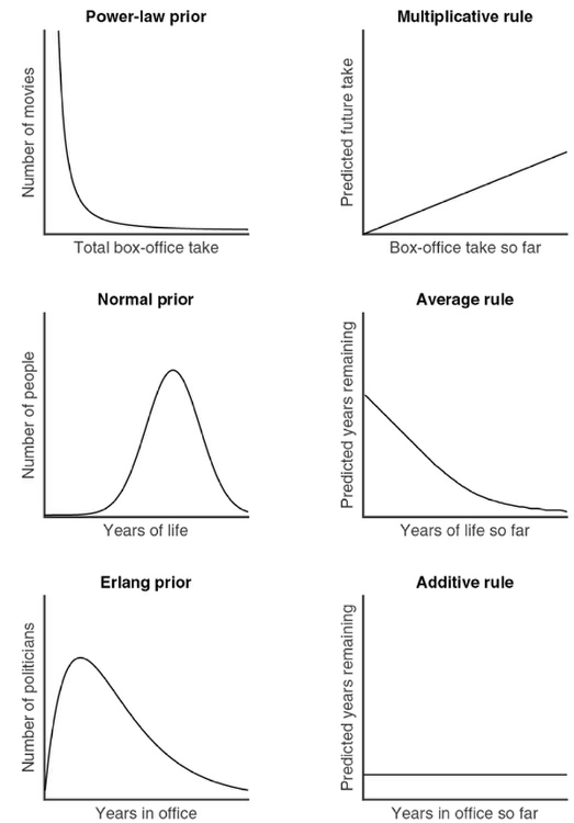
The three central varying patterns of optimal prediction are the Multiplicative, Average, and Additive Rules. People naturally know which distribution to use when predicting certain things as long as they have informative priors about the distribution they’re predicting. Thus people will be much more likely to accurately predict the average lifespan of a dog than a Galapagos Giant Tortoise; most people have more experience with dogs than tortoises.
This leads to my personal favorite conclusion of this chapter: people’s judgements are shaped by their expectations, which in turn are shaped by their experience. Thus, what people predict about the future betrays much about the person’s past experiences. This is becoming especially poignant with modern and mechanized technology, for people are able to absorb information in ways that aren’t necessarily true to how the world really is. People’s experiences are therefore being abnormally shaped by modern technology, which in turn is abnormally shaping their expectations of what will happen in this world, which in turn influences which judgements they will make, such as how they will vote or what beliefs they will hold. Modern technology, while having many, many positives, also unwittingly leads to many negatives as well.
Chapter 7: Overfitting
The subtitle of this chapter is “When to Think Less,” and that summarizes this chapter very well. Overfitting occurs when a function is too closely fit to an insufficient amount of data points. This appears counterintuitive; this argument calls for a modeled function to be less complex and include fewer factors than what might be possible. Through graphing different n-factor formulas for data that related the satisfaction of married couples over time, this chapter illustrated that the 1-factor formula provided a linear slope that would not be practical, and that a 9-factor formula was too unpredictable and would vary wildly even if one data point was slightly shifted. The sweet spot, for this data, happened to be using a 2-factor formula. This illustrated that considering too many factors can lead to overfitting, an important issue to avoid in machine learning.
In order to detect -and hopefully remedy- overfitting, cross-validation can be used. Cross-validation tests to see how well a model fits data it hasn’t seen, whether that is even less data than originally given or more. Let’s say, for example, we were to remove two data points from a data set of ten points. If we then tried to fit this new data set and realize the previous model wildly deviates from those two removed data points, then overfitting is probably playing its mischievous hand. Proxy metrics are also useful for cross-validation; using different tests to ensure the data is proceeding as expected is an important way to double-check models.
While cross-validation can detect overfitting, it does not remedy the overfitting on its own. Thus regularization is used to remedy the ugly beast of overfitting. Regularization is the use of constraints that penalize models for their complexity. It runs on the principle that, unless the more complex model does a significantly better job than a more simple model, the simpler model should be used. One famous complexity penalty algorithm is the Lasso, which determines its penalty by calculating the total weight of the different factors in a model. The Lasso brings down as many factors as possible to zero, simplifying the factors so that only the most impactful factors are left in the model equation. Penalty techniques such as the Lasso are now ubiquitous in machine learning, a field that I might? pursue in the future?
While modern life moves swiftly, machine learning and evolution occur slowly, which can actually be better than changing too swiftly, which can lead to overfitting. In order to prevent this swift descent into overfitting, the regularization technique known as Early Stopping can be used. As an example, fine-tuning the exact details of a lecture rather than focusing on the main points can lead to overfitting one’s lecture by focusing on the nitty-gritty details too much and thus losing the audience’s attention. Counterintuitively, thinking and doing less can lead to better decisions and outcomes if we were to take suggestions from machine learning’s use of effective regularization techniques.
Chapter 8: Relaxation
Chapter 8 discussed the concept of relaxation. Not the resting with cucumbers on your eyes relaxation, but the relaxation that allows otherwise impossible problems to be solved in a way that is close to the optimal solution. There are many problems out there which could be solved through brute force alone with the help of some powerful computers. This can literally take eons, however, so oftentimes using relaxation techniques to simplify these otherwise overly time-consuming problems is a must. There are also, of course, intractable problems that simply could not be solved without the use of relaxation techniques.
As an example of a problem which has no known optimal solution, the classic Traveling Salesman problem’s frustrating past was doled out. Despite all the Traveling Salesman problem’s history, there is no known efficient algorithm that definitely solves this problem. “Efficient,” or tractable, algorithms are defined as algorithms that are O(n^x), where x can represent any number, versus say a hefty O(2^n) algorithm. When algorithms reveal themselves as intractable, relaxation techniques become a necessity.
Three important relaxation techniques are discussed in this chapter: Constraint Relaxation, Continuous Relaxation, and Lagrangian Relaxation. Constraint Relaxation is true to its name; it simply removes, or “relaxes,” certain constraints to an algorithm so that it may become solvable before the true algorithm solution is sought after. Continuous Relaxation transforms discrete choices into fractional choices; rounding of the fractions can then lead to a close-enough-to-optimal solution. Lagrangian Relaxation aims to change impossibilities into penalties so that the rules can be bent appropriately enough for a near optimal solution to be found.
While relaxation techniques are not themselves as good as an optimal solution, they still retain many benefits. For one, they can offer a bound concerning what to expect from an optimal solution. This can be seen in the use of a “minimum spanning tree” in the Traveling Salesman problem, which uses Lagrangian relaxation-like techniques to swiftly come up with the optimal solution time despite not solving the problem itself. Relaxation techniques also retain the ability to be reconciled with reality well if done correctly.
Instead of brute forcing through problems which may literally be impossible, sometimes it is best to go with a near-optimal solution via relaxation techniques.
Chapter 9: Randomness
Chapter 9 argued for the benefits and effectiveness of randomness. This contrasts from the normally “deterministic” behavior we are used to getting from computers. To be sure, randomized algorithms will not lead to the optimal solution, but they will succeed in getting very near to them in a much shorter time span. The first given example of a randomized algorithm’s usefulness was the Monte Carlo Method, which relies on random samples to calculate its results.
The concept of certainty in computer science was also discussed and illustrated using Gary Miller’s equations, which yield a false positive every fourth attempt in its algorithm. Michael Rabin, a Princeton PhD, then helped pose the Miller-Rabin primality test, which provided a quick way to identify gargantuan prime numbers with an arbitrary degree of certainty. (The more correct attempts of prime numbers, the more likely the number is truly a prime.) This deviates from the typical mathematical concept of certainty -if we can are only sure that a number is prime with an arbitrary amount of certainty, is it worth the many brute force hours that we saved by not checking every single prime number leading up to that gargantuan number?
This chapter also gives the benefits of random sampling, which is shown to have great practical use both in political decisions and in philanthropic organizations. In addition, a third factor is considered in the tradeoffs of computer science along with the typically known factors of time and memory space -error certainty. Error certainty is explored through the Hill Climbing algorithm, which yields a visual example about local maximums and how a sampling a model can lead to contentment with a mere peak of a hill while there is a giant mountain off in the distance. Instead of stopping on the mere hill, considering other random data every time a decision is made in an effort to get to the highest peak could be used instead - this would be the Metropolis algorithm.
This chapter’s argument was pretty simple: randomness and uncertainty are sometimes necessary evils that will lead to the closest to optimal solutions as we can practically get; they should be used carefully and concisely.